Maze Navigation Using Cameras for Localization and Obstacle
Avoidance
Project 2, ME 597D Advanced Mechatronics
- Spring 2012
Saurabh
Harsh
John Bird
General Description of the Problem
The second project is to create a system to navigate the robot out of a maze using overhead cameras to determine robot location and the maze outline. The maze is outlined on the floor in red tape, except for certain regions which have no visually identifying regions, but are marked by physical walls with overhangs. Effectiveness of the maze solving implementation is evaluated by the time required for the robot to successfully navigate out of the maze, scattered throughout the maze are green chocolates which are worth ten seconds of time if carried out of the maze.
Equipment
The robot used throughout the course is also used for this project, pictured below:

The robot has two continuous rotation servos directly driving the front wheels, and a omni-directional roller in the rear. A central position-command servo can point a Sharp IR range finder to provide range/bearing information. Commanding the robot is an Arduino Uno R3 which communicates with the controlling computer via a Serial to USB interface.
For this project the robot is fitted with a L3G4200D rate gyro to allow feedback control on the commanded yaw rate, overcoming the difficulty associated with calibrating an open-loop turn rate by differential wheel speed. The gyro communicates with the Arduino via i2c which communicates the measured rate back to the controlling computer.
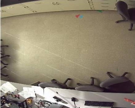
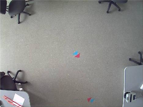
The lab is equipped with three IP cameras to allow the robot and walls to be located through vision processing. The vision of the cameras overlaps to allow continuous tracking of the robot as it transitions from one camera to another in the maze. The cameras have no correction for distortions or misalignment, leading to some mismatch in the transition zones. Maze walls are marked on the floor in red tape to allow visual identification. Sample images from two of the three cameras appears below:
The Arduino is set up to simply take servo pulse width commands from the computer, issue them to the servos, and report back the current Arduino time, servo pulse widths and measured yaw rate. Minimizing the processing occurring on the Arduino allows all of the command and control software to be written in MATLAB and run on the control computer. This approach reduces the performance and rate of some controller tasks by adding the serial interface and MATLAB overhead, but speeds development through use of the powerful MATLAB debugging tools, which is key to meet the short time period allotted for the project.
Organization
In order to allow parallel work and break the project into more manageable pieces, three task areas are identified and assigned:
|
Task |
Description |
Assigned To: |
|
Vision Processing |
Camera interface,
identification of robot location and orientation, as well as
wall locations |
Saurabh |
|
Path Planning |
Using robot and wall
locations, plan an efficient path out of the maze, generate
commands to the Arduino |
John |
|
Arduino Communication |
Send and receive data from the
Arduino over serial |
- |
The vision processing was involved reading in vision data from the IP cameras, segmenting the image into regions of interest based on color, and using the geometric charaacteristics of these regions and their proximity to other regions to develop useful information. In addition to identifying walls, the vision processing function rejects other robots, and identifies the region the robot is located in to speed later vision processing calls.
Path planning requires taking the occupancy grid from the vision processing step, running a path planning algorithm to determine feasibility of a path to the goal, and given feasibility, to calculate the fastest path. Once a path has been determined the path planner must determine the error in the robot's location and generate commands to put it back on the proper path.
Communication with the Arduino is re-used from a previous lab, and used a serial connection from the control computer to the Arduino, sending packets of binary data, with start sequences to identify the packet beginning and allow extraction of the message. Each message to the Arduino gives a command to send to each servo and included a checksum to verify message integrity. Messages from the Arduino include the time of transimission, acknowledge the servo commands, and include IR range and gyroscope rate information.
The three blocks in the project are implemented in a MATLAB gui for ease of use that display the current image data and the robot's environment as interpreted by the vision processing system. The path planned for the robot and its location is also displayed to aid the operator in verifying that the system is working as intended.
The vision processing, control, and Arduino communication functions run in MATLAB timer objects, allowing continuous running at a fixed rate. MATLAB does not offer true real-time operation, so the system has to to be robust to missed or delayed signals. Several steps, detailed later, are used to account for the lack of real-time operation.
Image Processing
Image processing uses the images
from three overhead IP cameras installed in the lab. An image from the
camera is obtained using an imread
command and it takes approximately 1/3rd of a sec for Matlab to execute the command. The image
processing section basically comprises of three parts:
1.
Identify
maze from the tape on the floor
2.
Determine
robot location
3.
Track
robot location and keep refreshing the correct camera
In addition to this the program
also identifies green candies on the floor though the downstream
control algorithm doesn’t use that information. Objects in the images
are identified based on their color and from the experience of
previous labs L*a*b color space was the obvious choice for the job. Matlab loads an
image as a 3 dimensional Matrix e.g. an image of 800x600 resolution is
a 800x600x3 matrix of unsigned integers(0-255) where the three numbers
for each pixel correspond to RGB values. While this format is very
easy to work with when it comes to identifying colors this format
doesn’t give correct results always because the RGB values for colors
change considerably with lighting conditions. The L*a*b space gets rid
of this anomaly since it provides absolute color information in
parameters a and b and Lightness(L) of the
color is separated from the actual color information. With a Cartesian
to polar conversion for a and b, R and
theta values can be generated where theta values corresponds directly
to the color as shown below in the color wheel.
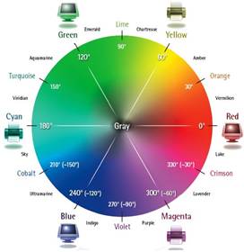
[http://uofgts.com/PS-P2Site/color_wheel.jpg]
However the color transform from
RGB to Lab is computationally intensive and hence should be used with
caution. The transform for a 800x600 image
takes approximately 1sec on a reasonably fast computer and processing
speeds of this order is not desirable while doing things like
tracking. Once the Lab data is created standard Matlab
functions like bwboundaries and regionprops
are used after thresholding the image for
appropriate theta values depending on what color one is looking for.
The program identifies objects mainly based on two parameters: area
and a roundness metric. More information
about bwboundaries and regionprops
function and how to use roundness can be found here.
During the first run of the program it loads images from all three
cameras and processes all three images to find out the maze
information by identifying red areas. Boundaries of areas which have a
metric of less than 0.3 are recognized as maze. The images from the
three cameras had considerable overlap and the maze was created by
adjusting the overlap using trial and error.
The fiducial
used for our robot consisted of a red and a green triangle placed next
to each other. The roundness for a triangle varied 0.3 to as high as
0.7 and the area varied from 150 to as high as 450. In case a red area
matching the description of the red triangle was found the program
could find green areas matching the description of a triangle and
determined the distance of the centroid
of the triangles. If the distance was found within acceptable limits
it was established that centroid of the
red triangle represents the location of our robot.
Once the robot’s location was found the function could
remember which camera was the robot found in and what was the location
of the robot. In the next run the program would refresh only that
particular camera and in that image look for the robot only in a 100
x100 cropped image around the last location of the robot. The L*a*b
transform for the cropped image took only 0.1s to run thus saving
tremendous amount of time. If the program could not determine the
location of the robot it would again refresh all images and start
looking for the robot in all images. The program is also designed to
correct barrel distortion in the images but the maze extended too far
to the sides of the image and the correction algorithm just neglects
the picture too much to the sides. Thus it was found better to go
without a corrector. Once the robot was found in the scene the Image
processing part could finish one cycle in about 0.4s while without the
robot in the field of view the processing time was approximately
4secs.
Path Planning
The path planning implements a D* lite-like algorithm (following the algorithm Dr. Brennan presented in class) to determine the optimal route from the robot's location to the goal. D* is chosen to allow fast path re-planning if an obstacle is discovered by the camera or IR sensor while solving the maze. The re-planning was never implemented however, due to difficulty gathering meaningful information about obstacles from the IR sensor. The IR sensor readings are very noisy and when combined with uncertainty in the orientation of the robot itself as well as the IR sensor relative to the robot (the IR pan servo takes a finite amount of time to travel to the commanded position), the IR sensor readings become very difficult to interpret. In the end the IR sensor is excluded from use in path planning and a path is simply planned at initialization and driven. This approach lends a danger of collision with another robot (the only obstacle that would appear after initialization), but if practice it was not a problem.
Before planning the path, the planning function first dilated the maze
by half of the "characteristic size" (in this case length) of the robot
(with a 10% safety factor), allowing the robot to be safely approximated
as a point mass moving in the maze. The effect of the dilation process
is pictured below:
 |
 |
The algorithm used was based on an algorithm presented by Dr. Brennan
is his lecture on path planning and operates as follows.
The algorithm plans initially from the goal to the starting location, initially assigning all nodes an infinite cost. The goal cell is examined first, and assigned a cost equal to the number of nodes transitioned in reaching that cell (the travel cost, in this case zero) added to a heuristic cost, defined as the maximum of the x or y distance from the goal. Once a cell is assigned a cost, the algorithm proceeds to the neighbor of the current cell which has the lowest heuristic cost.
The algorithm runs until there are no more unexamined cells which are valid robot locations or until it reaches the start point. In the former case it is then concluded that there is not a feasible solution to the maze. In the latter, the algorithm then finds the neighbor of the start point with the lowest assigned (travel plus heuristic) cost, adds that cell to the path and continues the process until the goal is reached.
It was originally intended to add a term in the heuristic cost to represent the value of picking up candies in solving the maze, but a lack of time to complete the project prevented this from being implemented.
An example of the output of the path planner is pictured below:

Once the path has been planning, commands are generated to steer the
robot to the path with the following algorithm:
1) The point on the path nearest the robot's location is determined
2) The mean of the next 6 points is taken to be the "current goal" of
the robot (6 was determined to be a good look-ahead amount by
experimentation)
3) The dot product between a vector in the robot direction, and the
diection of the "current goal" is used as an error term in the speed
command calculation (so if the robot is facing away from the goal it
backs up, facing 90deg it doesn't move, and facing the goal it goes full
speed)
4) The cross product of the robot and goal directions is used as the
error term in the turn command (though if the robot is facing away from
the goal then it saturates the turn rate in the direction nearest the
goal bearing)
The process is illustrated below.

Time constraints required the elimination of capturing candies as a goal in the path planning algorithm, no effort is made to capture them, though a catcher mechanism is fitted to capture candies that happen to be in the robot's path.
Since the vision data is processed at only 0.5 Hz, a model of the robot is run in the control loop to provide higher rate command updates, the model is then updated each time new vision data is available. The model uses the commanded speed (reported by the arduino) and gyro yaw rate measurement to determine the new robot state at each time step. Since MATLAB is not capable of providing true real-time operation, the time used to integrate the robot state comes from the robot itself. Each time a new data packet arrives from the Arduino, it contains the Arduino time in milliseconds, and this step is used in the model update, a similar process was used in a previous lab and showed performance considerably superior to using the MATLAB timer step size.
Arduino
Communication
The communication with the Arduino is
accomplished using the MATLAB serial object. Packets of serial data are
sent in binary mode, beginning with the sequence 255 255, and
ending with a checksum calculated as the XOR of all bytes in the
message. This structure allows both MATLAB and the Arduino
to send data without handshaking, so that the unpredictable timing of
MATLAB read/write executions does not cause the interruption of the
program on either end. Sending only servo commands to the Arduino
allows all controllers to be written (and tested) in MATLAB, speeding up
development substantially.
Testing
To allow the path planner and controller to be tested independently of
the vision data a maze generation and robot simulation program was
written. This allows random mazes to be generated and the robot to be
driven through the maze in simulation, speeding up testing and allowing
the path planner to be tested on more and more diverse mazes. Examples
of mazes generated are pictured earlier in describing the path planner.
The simulation is set up by adding another timer to simulate the robot
to the matlab gui, replacing the vision processing. The robot can then
be driven as a hardware in the loop simulator allowing easy debugging
without having access to the vision data, and allowing debugging to
occur before the vision processing element is complete.
Performance
In testing, the system is found to have good performance, capable of finding a path out of the maze and navigating along that path. During the class competition the robot was capable of navigating out of the maze in under 2:30. Though several attempts did result in contact with walls, the controller is largely capable of keeping the robot in free space.
Software
The maze generation and path planning example software is linked here (note that the final D* function implemented in full code has some bug fixes and speed-ups that are not implemented here).
Full gui and robot communication code is linked here (not very clean or well commented, but it's there - runController is the gui initialization function).
Arduino code for robot communication is linked
here.