Background Model
A linear model is used to update the background to include slow time-scale changes in scene being observed. The linear model is explained below:
y_n= αy_(n-1)+(1-α) x_n
y_n is current model of the background,
y_(n-1) is the previous step model of the background,
x_n is the current Range data from the sensor,
α is the learning parameter which decides how quickly the model must change with the change in surroundings (higher α implies slower learning).
In the current project work we used α=0.999, which is ideal to use in cases where we have dynamic environments and we wish to localize an object even if it stops moving for a considerable amount of time.
Object Detection
Once a new scan is obtained and the background model has been updated, in order to detect any changes in the scene, the new range data (x_n) is subtracted from the background model (y_n) to obtain the error vector(e_n).
e_n=x_n-y_n
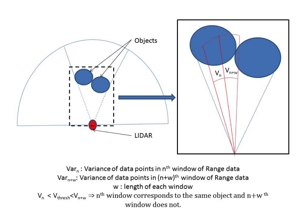
A window of length w≪length of x_n is moved across e_n and for each location of this window the mean of this error value is estimated and is compared with a predetermined threshold. If error is higher, than, this threshold then, it means that, there has been some significant change/movement at the location of that window. Location of the window is defined as the center of that window. Now, the variance in this window corresponding to the data in x_n is estimated to determine whether all points in the window belong to the same object. If the points do belong to the same object, then, variance should be small. If the window is at the region of overlap of two objects then, variance would be higher as demonstrated in the figure below. This technique allows us to distinguish between two very close moving objects.
e_n=x_n-y_n
A window of length w≪length of x_n is moved across e_n and for each location of this window the mean of this error value is estimated and is compared with a predetermined threshold. If error is higher, than, this threshold then, it means that, there has been some significant change/movement at the location of that window. Location of the window is defined as the center of that window. Now, the variance in this window corresponding to the data in x_n is estimated to determine whether all points in the window belong to the same object. If the points do belong to the same object, then, variance should be small. If the window is at the region of overlap of two objects then, variance would be higher as demonstrated in the figure below. This technique allows us to distinguish between two very close moving objects.
Object Tracking and Estimation
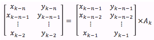
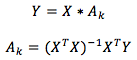
We first address the case of single object tracking with obstacles. In this case, we repeat the process of object detection to update the position of the object in each step. This process is essentially, the object tracking, but, it will work as long as the object is visible to the sensor. In order to facilitate trajectory estimation of the object, we all need to predict the location when the object is not visible to the sensor. This prediction is done on the basis of a discrete time linear equation:
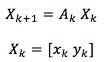
(x_k,y_k) is the position of the object at kth instant.
Model Prediction: Ak is a 2x2 matrix, which is estimated as the least square estimate of Ak using previous ‘n’ values of Xk.
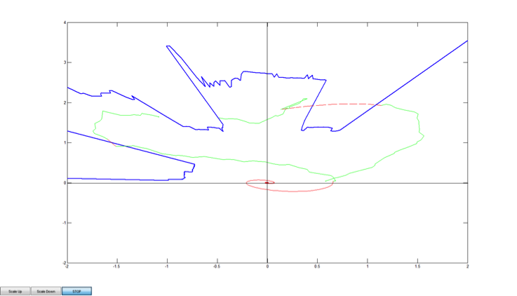
Comments on Stability of the Model: Looking at the construction of Xk , we know that, the estimated trajectory is nothing, but, an orbital path of the system in the phase space with xk and yk as the two states. The stability of this model, does not affect the tracking performance directly. But, the following observations were made in relation to the stability of eigenvalues:
1. If both eigenvalues are beyond the unit circle, then the path tends to go away from the origin (i.e. location of the LIDAR) very quickly, as the system is unstable.
1. If both eigenvalues are beyond the unit circle, then the path tends to go away from the origin (i.e. location of the LIDAR) very quickly, as the system is unstable.
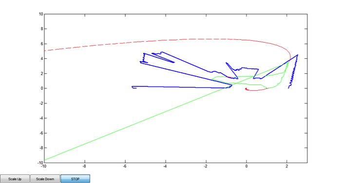
2. If both eigenvalues are within the unit circle, then the path tends to go towards the origin and slows down while doing so.
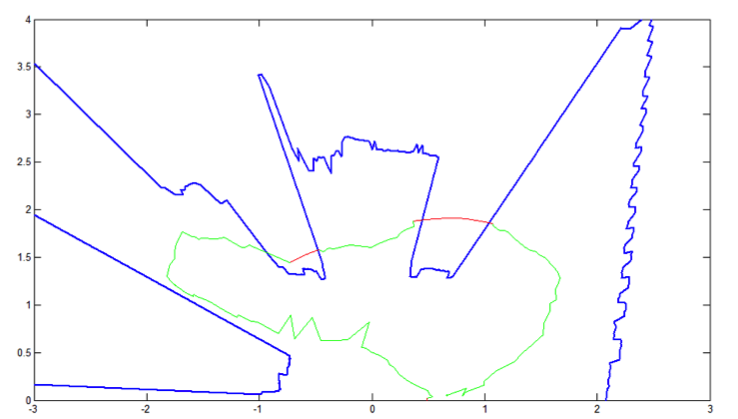
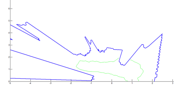
Results
1) Tracking Object (green line)
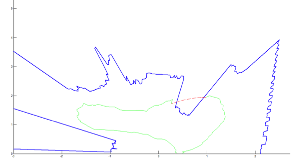
2) Tracking objects with trajectory estimation
3) Tracking object with trajectory estimation: Case of 2 obstacles